A dynamometer result describes power and torque at a stated measurement boundary, under a stated test procedure. A number labelled “power” can be measured at an engine coupling, at a hub, or through a tyre and roller; an estimated crankshaft figure is a calculation rather than a direct engine-dyno measurement. See the dynamometers overview for the different layouts.
Torque, speed and power
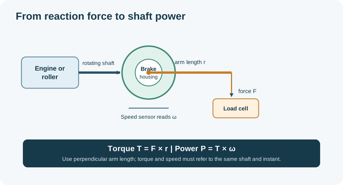
Torque is the turning effect at a shaft. A common absorber has a casing that can react against a load cell through a known lever arm: torque is force multiplied by the perpendicular arm length. Shaft speed is measured separately, and mechanical power follows from torque multiplied by angular speed. For torque T in newton metres and speed n in revolutions per minute: power (kW) = T × n / 9,549. With torque in pound-feet, mechanical horsepower = torque × rpm / 5,252. These figures use the torque and speed at the same shaft and the same instant. At 400 N·m and 3,000 rpm the calculation gives approximately 125.7 kW, or 168.5 mechanical hp. Metric PS is a different unit; 1 kW is approximately 1.360 PS. Sources: SuperFlow: engine dynamometer measurement and US Department of Energy motor systems sourcebook.
A graph may label torque against engine rpm even when the measurement is at the rollers. Gear ratio and tyre or roller geometry are then involved in translating the displayed speed and torque. Do not substitute wheel torque into a formula with engine rpm. Check the instrument’s definitions, rpm pickup and units.
What is included in the result?
- Engine dyno: the coupling measures output from the engine as installed on the stand. Its accessories, exhaust, intake and correction standard must be stated before comparison with a manufacturer rating.
- Hub dyno: the load is applied at the wheel hubs, downstream of the transmission and differential but without tyre-to-roller losses.
- Rolling road: the driven tyres turn rollers, so the displayed wheel or roller result includes losses in the driveline and tyre/roller interface. See Dynojet: wheel and crank horsepower.
Losses vary with the vehicle, temperature, speed, gear and load. A fixed percentage is an assumption, not a measurement of a particular vehicle’s loaded driveline loss. A chassis dyno’s estimated flywheel figure should be labelled as estimated; its method and correction should accompany it.
Sweep, steady state and inertia
In steady state the speed is held approximately constant while the load cell measures reaction force. In an accelerating sweep, some output also accelerates the engine, couplings, rollers and other rotating parts. An inertia dyno calculates energy and power from the acceleration of known inertia; a load-controlled system may combine absorber torque with an inertia term. Compensation and test method differ between systems. Acceleration rate changes the result, and a rapid sweep can give different results from a held point. SuperFlow: determining engine and dynamometer inertia.
Coastdown and corrections
Coastdown records deceleration after driving torque is removed. Depending on the procedure it can check dynamometer parasitic loss, characterise a vehicle’s road load, or feed a chassis-dyno loss estimate. Those are different tasks. Road-load coastdown includes aerodynamic, rolling and other resistances, and emissions test procedures derive the load the dynamometer must simulate after allowing for losses still present on the rig. It does not prove that deceleration losses equal loaded driveline losses. See US EPA: vehicle road-load force and dynamometer settings and EPA research on separating coastdown losses.
Atmospheric correction uses a named method and measured conditions to report a standardised value. The uncorrected result remains useful: retain both, the correction method and factor, pressure, temperature and humidity. A correction cannot eliminate all effects of heat soak, charge-air temperature, calibration changes or equipment differences. Dynojet: applying correction factors.
Calibration and fair comparisons
Follow the equipment maker’s zero, span, speed and verification procedures. A known, traceable weight and calibrated arm can check a reaction load cell; speed requires its own check. Dynamic checks and coastdown checks address different parts of the measurement chain. The EPA dynamometer quality-control guidance describes dead-weight checks and coastdown for a particular emissions-test programme; use the requirements applicable to the machine and intended test.
For a before-and-after comparison, record dyno and software, correction, measurement boundary, gear, test mode and sweep rate, tyre pressures and restraint setup, fuel, cooling, ambient and intake conditions, and engine temperatures. Warm consistently, allow recovery between pulls, check for tyre slip or vehicle intervention and repeat runs. Compare the whole curve and uncertainty, not just one peak. A repeatable small change can still be smaller than measurement uncertainty. SuperFlow: dynamometer testing oversights.
Reading a power and torque graph
A graph should state its power unit, torque unit, horizontal-axis source and measurement boundary. Mechanical horsepower, metric PS and kilowatts are different units. The peak torque and peak power normally occur at different speeds, and their values must not be inserted into the same power equation unless they were recorded at the same speed. With torque in N·m and speed in rpm, power (kW) = torque × speed ÷ 9,549.3. A displayed torque curve against engine rpm may have been converted from measured roller or hub torque using a measured or assumed ratio.
For a multi-hub machine, calculate each measured hub's instantaneous power from its own torque and speed, then add simultaneous signed powers as appropriate. Wheel speeds can differ, especially with a differential or electronic torque distribution; multiplying the sum of torques by a single unrelated speed may give a misleading result. Retain both original channels and the software's sign convention. In an engine-test context, the US EPA work-determination procedure describes synchronising speed and torque before calculating instantaneous power.
What a calibration checks
Calibration relates the indication to known reference values under specified conditions; repeatability alone does not show that a sensor reads correctly. A reaction-arm load-cell check normally compares indicated torque with force applied through the specified perpendicular arm. For illustration, a 20 kg mass under standard gravity (approximately 9.80665 m/s²) applies approximately 196.1 N; at a 0.500 m perpendicular arm that represents about 98.1 N·m. This is an example of the calculation, not an instruction to use a particular arm, weight or setup. The mass, arm length, orientation, tare, friction and any correction must match the equipment maker's method.
Check zero and span at the specified points and in the appropriate directions where relevant; a single point does not establish the whole system's linearity or dynamic response. Only perform the check with the machine stopped and in the condition required by its instructions. A weight and arm test exercises the installed force-measurement chain; it does not by itself verify speed pickup, roller inertia, time alignment, atmospheric sensors or the correctness of the report calculation. SuperFlow discusses verified calibration weights; its WinDyn manual notes that zeroing with an active applied load shifts the reference.
Speed checks should use a suitable reference and the installed pickup's pulse count, trigger wheel and gearing. Inspect and record the calibration procedure, reference instruments, as-found and as-left results, and the next verification date according to the facility's requirements. Acceleration and transient checks can reveal issues that a static load-cell check cannot. Do not apply acceptance tolerances from one dyno or test standard to another without checking their scope.
Repeatability, uncertainty and small changes
Repeatability is the closeness of results obtained under similar conditions; measurement uncertainty describes the range reasonably associated with a result after considering relevant sources. These are related but different. Calibration, drift, speed and torque sensing, filtering, test rate, fuel and temperature all contribute. A short series of repeat pulls can reveal instability, but its range alone is not a complete uncertainty estimate.
For example, baseline peak results of 248, 250 and 249 hp have a mean of 249 hp and a range of 2 hp. If a later run reads 251 hp, its 2 hp difference from the baseline mean is comparable to that observed range. That observation alone cannot establish whether the modification caused the difference: make further matched repeats, review whole-curve behaviour and changes in operating conditions, and quantify uncertainty as appropriate. Do not treat the example range as a confidence interval or a universal pass/fail threshold.
Where practical, use matched baseline and changed tests, consistent warm-up and recovery, and multiple runs. If changes can be reversed, an A–B–A comparison helps expose drift. Keep an audit trail of the raw and corrected curves, fuel, gear, tyre and restraint setup where relevant, temperatures, ambient conditions, test type, sweep rate, calibration and software version. SuperFlow's test guidance discusses temperature consistency, acceleration rate and calibration.
Sweep rates, inertia and filtering
During acceleration, part of the available torque accelerates the engine and test equipment. A simplified inertia contribution is T = I × α, where I is the relevant mass moment of inertia and α is angular acceleration, expressed at the same shaft. Gear ratios and additional rotating components complicate the calculation; losses and the installed controller's reporting method still matter. Some dynos apply inertia compensation or correlation, while other results show measured brake output without that adjustment. State which convention is used.
Match the test rate and method before interpreting small changes. A steady-state point, a controlled ramp and a free inertia pull do not necessarily exercise the engine, turbocharger or temperatures in the same way. Filtering and graph smoothing can hide noise but also alter the appearance of sharp peaks; identify the same smoothing settings and compare raw channels where needed. SuperFlow: acceleration effects; engine and dyno inertia.
Diagnosing a surprising change
- Different curve but similar peak: compare the full usable speed range and verify matching gear, engine-rpm source and graph scaling. A shifted RPM signal can move both curves.
- Power varies between pulls: compare intake, coolant and oil temperatures, boost and ignition or ECU intervention where available; check fuel supply, tyre contact and consistent cooldown as well as atmospheric correction. A correction factor cannot restore a heat-soaked intake or a different control strategy.
- Wheel, hub and estimated crank figures differ: confirm the measurement boundary, test method and correction. Coastdown estimates or fixed loss percentages are model-dependent and are not direct measurements of loaded drivetrain loss.
- Sudden spikes or implausible torque: check pickups, sensor mounting and wiring, signal scaling, wheel slip, data timing and any recorded fault before attributing them to the engine. Investigate the raw data; smoothing a spike is not a repair.
See also controller hardware and control modes and test setup and safety.
For practical checks of the torque arm, speed and environmental channels, see dynamometer calibration and verification.
For a practical guide to reading a printout, see dyno graphs explained: torque and horsepower calculations, what is measured and why results differ.